FAQ
How does the scanner trigger my stimulus program?
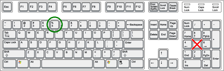
When the scanner starts acquiring data the stimulus computer will receive the same signal as if the “5” has been pressed in the top number row of the computer keyboard, as illustrated in the picture (NOT the “5” in the numeric keypad, that is a different signal). Pressing the “5” in the top number row on any computer is IDENTICAL to the trigger signal received from the scanner by the stimulus computer, therefore for trigger testing purposes it is not necessary to connect to the scanner set-up.
What is the slice acquisition order for functional scans?
Slices are acquired in an interleaved fashion from inferior to superior (i.e. bottom of the head to the top) assuming you have an axial or oblique axial acquisition (which is usually the case). If you have an odd number of slices, the lowest slice will be the first to be acquired (i.e. slice 1), whereas if you have an even number of slices, the second to lowest slice will be first (i.e. slice 2). For example, if you acquire 7 slices the order of slice acquisition would be [1 3 5 7 2 4 6], whereas if you acquire 8 slices it would be [2 4 6 8 1 3 5 7].
Note that the slice order is complicated by the use of sms (simultaneous multi slice, aka mb, multi band). The dicom header for functional scans will include the exact timing for each slice. Modern dicom conversion software, e.g dcm2niix, will translate these values into a json file as a “Slice Timing” entry in BIDS style, which can then be used with modern slice timing correction tools.
How long should my functional scan be?
The length of a functional scan is entirely dependent on the length of your paradigm. This being said, when developing the structure of your scan session/paradigm, it should be kept in mind that it is generally better to have a greater number of shorter scans than a smaller number of longer scans. This is mainly for two reasons: 1) longer scans are more prone to subject fatigue, and 2) in the event of a technical malfunction in the middle of a scan, less data will be lost when using shorter scans. Typical lengths for functional scans range from 6-10 minutes. Triggers are actually sent at the beginning of each frame (i.e. every TR), though it is most often only the trigger of the first recorded frame that is of interest for synchronization.
How many frames should I ignore in BOLD imaging?
With a TR of 2s, the standard BOLD sequence ignores the first two frames of every scan (i.e. these frames are not recorded; these are called “dummy scans” this value depends on the TR, so if you have a different TR please inquire further with Jacob), meaning the first trigger is actually sent at the beginning of the third frame, which is the first frame whose data is actually recorded. This should suffice, and therefore no extra frames need be ignored, however, if it is of concern, ignoring another 2 frames would be more than enough (though this would have to be appropriately taken into account in the corresponding analysis). The exception to this rule is Multi-Band EPI Data. For very low TRs (<500ms), steady state is not reached after the built in dummy scans. Programming your stimulus and analysis to skip the first ~10 frames is likely important. This may change in the future if we gain the ability to alter the number of built in dummy scans.
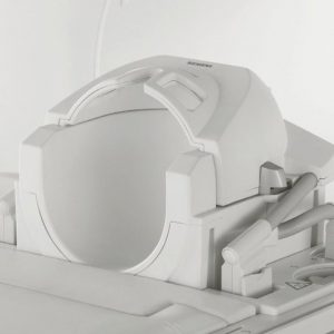
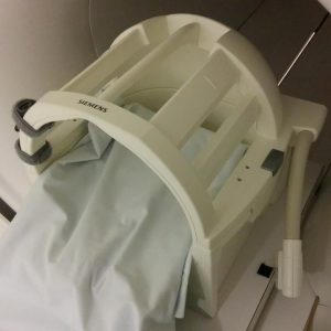
What are the differences between the three head coils?
What is the resolution, aspect ratio, and visual angle of the projector in the scanner?
A custom in-bore screen from VPixx is used just inside the back of the bore. This allows for the greatest FOV while maintaining a full unclipped rectangular image. It is also shaped and positioned to allow simultaneous use of our other systems, including allowing line-of-sight for our eye-tracker camera and leaving room behind the head coil for our EEG amplifiers.
The projection surface measures 44cm x 24.5cm. The projected image is just slightly smaller than that at approximately 43.5cm x 24cm. With slight drift in the projector position/angle over time, it’s possible to have the extreme edges of the image cut off by the frame. Although we check for this regularly, it’s safest to avoid using the extreme edges of the display for stimuli (about 10 voxels or 2mm).
The eye-to-screen distance is approximately 98cm. This will vary depending on subject head size, which will impact:
a) how close to the top of the coil (z-direction) the subject’s eyes are and the corresponding mirror position, resulting in a mirror-to-screen distance between 86 to 90cm (approximately 88cm on average).
b) how high up in the coil (y-direction) the subject’s eyes are and the corresponding required padding, resulting in an eye-to-mirror distance between 8cm and 12cm (approximately 10cm on average).
At the edges of the display the vertical FOV is approximately 14.5 degrees and the horizontal FOV is 25.8 degrees.
If the visual angle of particular images you’re displaying is of critical importance to your experiment, contact Jacob Matthews after your experiment is programmed but before you begin your pilots to arrange a time to confirm the correct display of your stimuli. In this context it may also be important to consider if the structure of the head coil is impeding vision of any particular section of the display, as this may unintentionally create monoptic viewing conditions.
What are sms/mb, ipat/grappa, and pf acceleration methods? What are the advantages/disadvantages?
Simultaneous Multi Slice (sms, aka Multi Band, mb) is a method of accelerating multi-slice 2D EPI sequences, i.e. fMRI or dMRI. By simultaneously exciting multiple slices distributed evenly throughout the FOV, and using some fancy tricks to disentangle the resulting overlapping readout data, the time to acquire a given FOV can be reduced by a factor of 2-12 (2-4 is typical, higher factors have exponentially increasing trade-offs). This can be used to reduce the TR of the scan, or traded off to e.g. use a finer resolution. The trade-offs of this acceleration fall into three main areas. There is a small SNR cost. There is also some potential cross contamination of signal between simultaneously excited slices (often measured as a g-factor). Both of these scale exponentially with acceleration factor. At low factors of 2 or 3, these costs are often so small that the acceleration is almost considered free. 4 is often used, but might be considered borderline. Factors above 4 are typically avoided, but evaluation of images might be worthwhile for specific use cases, such as very low TR imaging. As with parallel acceleration (below), a reference image acquired at the beginning of the scan is used in the reconstruction, potentially increasing motion sensitivity. It is also worth pointing out that slice timing becomes rather complex with sms imaging, requiring the use of modern dicom conversion software to extract the slice timing values from the dicom headers, and modern slice timing correction tools which can accommodate these slice timings. Outside of slice timing, sms imaging should not require any other special considerations in analysis.
iPAT (integrated Parallel Acquisition Technique) is the Siemens implementation of the parallel imaging technique, GRAPPA. Parallel imaging exploits the multiple channels of the head coil and their different spatial sensitivities to allow for the acquisition of a reduced data set while maintaining image quality. This reduction in acquired data can then allow for faster, higher resolution, or larger coverage scans. Also, due to reduced readout time, the minimum TE is lower, and EPI based distortions in both fMRI and dMRI are reduced. However, the use of parallel imaging results in a reduction in SNR, can result in an increased sensitivity to motion, and if used too strongly can result in artifacts. There is also a noted tSNR impact, disproportionately affecting deep brain areas, but also with some impact in peripheral cortex. As such, the use of iPAT for functional scans should generally only be considered when one needs to push either spatial resolution below the typical value of ~3 mm, or make the TR much shorter than 2 s, both while maintaining whole brain coverage. With the advent of sms acceleration, iPAT is required only to achieve very specific parameter sets, and is otherwise avoided.
Partial Fourier is a simple acceleration method which takes advantage of symmetries in k-space to reduce the readout time required for a given FOV. This is usually used in combination with one or both of the above methods when a lower TE is desired. Overall scan time can also be reduced, but not as drastically as with the above methods. The trade-off is slightly reduced SNR and a slight smoothing effect in the image.
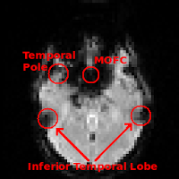
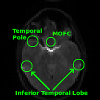
What regions are typically affected by susceptibility effects in gradient echo BOLD?
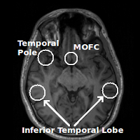
Regions commonly affected by susceptibility artifacts in gradient-echo BOLD include the medial orbitofrontal cortex (MOFC), temporal poles, and inferior temporal lobe. If your interest is particularly in one of these areas you may consider running a spin-echo BOLD scan, instead of gradient-echo, as it is unaffected by susceptibility effects.
How do I use/interpet the physiological (physio) recordings?
The easiest way to use the physio recordings (.ext, .puls, .resp) are to first process them using the prepphysio script that exists on most Rotman servers. prepphysio will “Preprocess Siemens physiological data dump files and convert them into a simpler format usable by AFNI and pretty much any other software.” For more information on how to use the script, just run the prepphysio command without any arguments on one of the servers and it will output instructions on how to use it.
In the case that prepphysio outputs the error “Was the scan only 1 measurement long? Did you even scan? There were fewer than two external reference timing triggers in 1fmri1214592.ext. It is not possible to match the physio data with a scan. Stopped at /opt/prepphysio line 211.”, this may indicate that the scanner triggers were not recorded correctly (you can check the .ext file; if there are no “5000” values written in the first line, then the scanner trigger was not recorded), possibly due to a bad connection during the scan. If this is the case, prepphysio will not be able to process the physio files as it no longer has a usable trigger recording which it needs to sync the physio recordings to the scan. In this event, you should still be able to manually process the physio recordings and sync them to the scan (see below), though this is less desirable. The physio files are structured as follows:
| 1 2 40 280 1026 1126 5000 1340 1653 … 1778 1800 5000 1774 1763 5003
ECG Freq Per: 0 0 PULS Freq Per: 73 813 RESP Freq Per: 0 0 EXT Freq Per: 30 1997 ECG Min Max Avg StdDiff: 0 0 0 0 PULS Min Max Avg StdDiff: 813 813 813 0 RESP Min Max Avg StdDiff: 0 0 0 0 EXT Min Max Avg StdDiff: 0 0 0 0 NrTrig NrMP NrArr AcqWin: 0 0 0 0 LogStartMDHTime: 60319027 LogStopMDHTime: 60768902 LogStartMPCUTime: 60317860 LogStopMPCUTime: 60768825 6003 |
Orange: Initial header information
Black: Recorded raw data Red: Trigger or other events (i.e. pulse/respiratory peaks) placed in with the raw data Green: Statistics Blue: Timing information Pink: Marks end of recording (5003) and file (6003) |
To manually extract the physio data from the .resp and .puls files, carry out the following steps:
- Read in the first row of the file and ignore/remove: a) the header information (orange above), and b) Any instances of 5000 (red above) or higher (e.g. 5003). You should then be left with the raw physio recording.
- The start and end times of a given physio recording are given, in msec from midnight (i.e. 0 would refer to 12AM), by LogStartMDHTime and LogStopMDHTime respectively. The start time of a given fMRI run can be found in the header information of that run’s first DICOM (if you don’t have a way to see DICOM header information, try ImageJ; when you open a DICOM ImageJ, click Image -> Show Info…). In the header, it will be found under the heading “0008,0032 Acquisition Time:” and will be in a 24h clock format (e.g. 165445.652500 = 16h 54m 45.6525s); you may want to convert it to msec from midnight.
- Using the two start times, find the point in the raw physio recording (from step 1) at which the run starts (Note: The physiological recordings are sampled at 50Hz, i.e. each sample is 0.02s after the previous). You can calculate the number of physio samples to include from this sync point on by using the TR and number of frames in your fMRI run (e.g. if your TR = 2s and you have 192 frames, then you will need to take a total of TR*number of frames/physio sample period = 2*192/0.02 = 19200 samples).
- Write the synced time course of physio samples into another file. If you want the file to be in the same format as output by prepphysio make sure that you save them into a text file with one value per line and save the text file with a .1D extension (i.e. run1.puls.1D, run1.resp.1D). NOTE: The default output of prepphysio for the .puls.1D file is to contain a time course that does not contain the raw pulse signal, but rather one that indicates the peak point of each pulse beat with a ‘5’, and ‘0’ everywhere else. If you are attempting to recreate the default output of prepphysio you will have to take this into account (i.e. you will have to find the peak points for the pulse time course, either manually or with a peak detector (e.g. in MATALB)).
For further questions please contact Jacob Matthews.